The Curious Case of Case When
Apr. 24, 2021While this post may only make sense for the graduate students who were enrolled in Dr. Kyla Dahlin’s graduate GEO 837: Applications Terrestrial Remote Sensing class, it is fairly easy to produce a land cover classification map in R with a .tiff file if land cover designations were classified a priori and determined or known by the user.
For example, I obtained my .tiff image after running a Random Forest algorithm for my scene of interest in Google Earth Engine, Phnom Prich Wildlife Sanctuary in Cambodia. During class, I remembered that I assigned a land cover value of 1 that corresponded to water, 2 corresponded to agriculture, 3 corresponded to canopy and 4 corresponded to clouds. Finally, 0 corresponded to NA values. Read about classification in Google Earth Engine here.
We use a combination of the stars and tidyverse packages and work flow to help us plot our land cover maps. The stars package attempts to serve as an
“update” to the tried and true raster package, and is way more friendly to tidyverse work flows, which is why I’ve chosen to adopt it. BUT your raster skillz should still be adept, as it is still the main R package when analyzing spatial raster data in R.
library(tidyverse)
library(here)
library(magrittr) # used for double pipe assignment operator
library(stars)
Notes: I use the double assignment operator in my work flow, read about %<>% here. The double pipe basically acts as a normal pipe, then updates the object simultaneously without having to change the name. I also use the here() function to locate my files. Jenny Bryan explains why you should use here(). This also is will not be most accurate land cover map, as this was a product of a Google Earth Engine intro to classification exercise.
I use the stars package to load my .tiff file.
ppws <- read_stars(here('data','phnomprich_landsat2020_RF_image.tiff'))
ppws # take a quick look
## stars object with 2 dimensions and 1 attribute
## attribute(s), summary of first 1e+05 cells:
##  phnomprich_landsat2020_RF_image.tiff
##  Min.   :0.00000
##  1st Qu.:0.00000
##  Median :0.00000
##  Mean   :0.04834
##  3rd Qu.:0.00000
##  Max.   :3.00000
## dimension(s):
##   from   to  offset        delta refsys point values x/y
## x    1 2355 106.512  0.000269495 WGS 84 FALSE   NULL [x]
## y    1 1843  13.001 -0.000269495 WGS 84 FALSE   NULL [y]
The key here is to know what’s going on with your stars object. We know that the stars object has 2 dimensions, which is our longitude and latitude (x, y) information. In each cell, there is 1 attribute, which is our land cover values that we knew of beforehand. This forms the basis of a raster image. We also can look at other information, such as the coordinate reference system and max and min values for latitude and longitude.
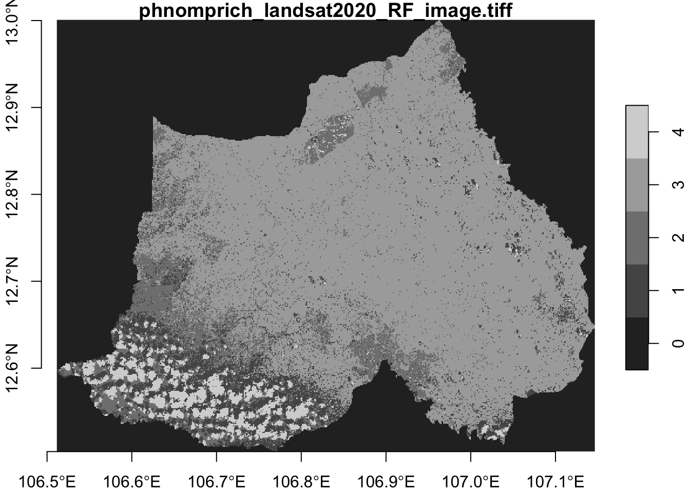
I can also use the plot() function to take a simple look at my tiff image. Note the legend and corresponding attribute values.
plot(ppws, axes = TRUE)
An easy way to check the values from our stars object dimensions is to use st_get_dimension_values(). Remember, the attribute values inside the cell does not form a part of the dimensions of the object (we have 2). If we had time-series data of multiple days and they were stacked on top of each other (like a brick) then that would introduce a third dimension (coming in a future post).
We can also double check the dimensions and names of our stars object if we’re still iffy on the stars object information. We can check for the names of the attribute values, and update if need be. Below, I update the name from “phnomprich_landsat2020_RF_image.tiff” to “value”. I save the column name “landcover” for later.
ppws %>%
  st_get_dimension_values(1) %>%
  head() # vector of longitude values
## [1] 106.5117 106.5119 106.5122 106.5125 106.5127 106.5130
ppws %>%
  st_get_dimension_values(2) %>%
  head() # vector latitude values
## [1] 13.00082 13.00055 13.00028 13.00001 12.99975 12.99948
dim(ppws) # 2 dimensions - x and y
##    x    y
## 2355 1843
ppws %>%
  names()                    # this name is cumbersome and long; time to change
## [1] "phnomprich_landsat2020_RF_image.tiff"
names(ppws) <- "value"       # update name for attributes
ppws %>%
  names()                    # check updated name
## [1] "value"
Another way I like to check and make sure everything makes sense is to look at our stars object in the form of a tibble/data frame. Let’s go ahead and do that:
ppws %>%
  as_tibble() %>%
  slice_sample(n = 10) # selects a random sample of 10 rows
## # A tibble: 10 x 3
##        x     y value
##    <dbl> <dbl> <dbl>
##  1  107.  13.0     0
##  2  107.  12.9     0
##  3  107.  12.7     3
##  4  107.  13.0     0
##  5  107.  12.9     0
##  6  107.  12.7     3
##  7  107.  13.0     0
##  8  107.  12.6     1
##  9  107.  12.5     1
## 10  107.  12.9     3
Okay cool, we now are pretty darn sure each (x,y) row has a corresponding landcover value. We can now use the combination of the mutate() and case_when() functions to create the land cover assignments. You can also create a new column with base R subsetting and indexing, but since I just started using R last year, I’ve been too ingrained in tidyverse ways and sipping the kool-aid. I also went ahead and created a “year” column just in case. The beauty of the stars package is to take advantage of tidyverse work flows.
# mutate new columns
ppws %<>%
  mutate(year = 2020,
         landcover = case_when(
           value == 1 ~ "water",
           value == 2 ~ "agriculture",
           value == 3 ~ "canopy",
           value == 4 ~ "clouds"))
Again, I make sure things are looking okay:
names(ppws)
## [1] "value" "year" "landcover"
ppws %>%
  as_tibble() %>%
  slice_sample(n = 10)
## # A tibble: 10 x 5
##        x     y value  year landcover
##    <dbl> <dbl> <dbl> <dbl> <chr>
##  1  107.  12.8     3  2020 canopy
##  2  107.  12.8     3  2020 canopy
##  3  107.  12.9     0  2020 <NA>
##  4  107.  12.6     3  2020 canopy
##  5  107.  12.6     0  2020 <NA>
##  6  107.  12.7     3  2020 canopy
##  7  107.  12.8     0  2020 <NA>
##  8  107.  12.9     3  2020 canopy
##  9  107.  12.8     3  2020 canopy
## 10  107.  12.8     0  2020 <NA>
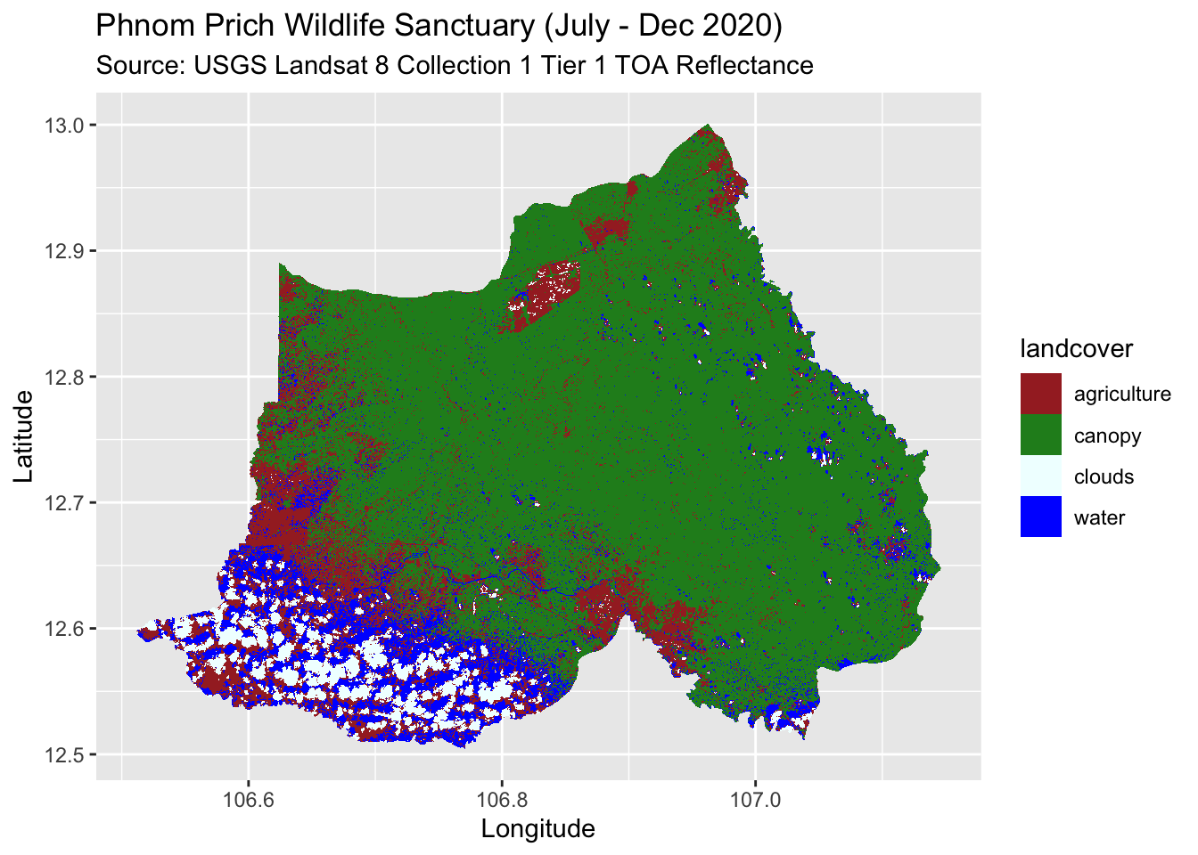
Okay, now I can use the geom_stars() function with ggplot() and use our “landcover” column values for aesthetics!
I create up a landcover palette. The colors will follow the alphabetical order of our landcover classes, so first should be brown, which I want to represent as agriculture, and so on. I also use the na.translate = FALSE argument so NA values get omitted in our ggplot. Ta-da!
landcover_pal <- c("brown","forestgreen","azure","blue")
ggplot() +
  geom_stars(data = ppws,
             aes(x = x, y = y, fill = landcover)) +
  scale_fill_manual(values = landcover_pal,
                    na.translate = FALSE) +
  labs(title = "Phnom Prich Wildlife Sanctuary (July - Dec 2020)",
       subtitle = "Source: USGS Landsat 8 Collection 1 Tier 1 TOA Reflectance",
       y = "Latitude",
       x = "Longitude")