xy: Plotting (Leopard) Locations in R
May. 3, 2021
One of the first steps in exploring spatial analyses with R is to produce a map with recorded (x, y) locations; for example, many researchers in wildlife biology mark animal locations with a handheld Garmin GPS and would like to see on a map where all the occurrences of their animal locations have been recorded. I remember it took me forever just to learn this basic exercise so I thought it would be a nice blog post for students in the same position and beginning their spatial journey in becoming a SAP (Spatially Aware Professional).
For #InternationalLeopardDay, I thought it would be a fun and simple exercise to download recorded leopard (Panthera pardus) occurrence records from the GBIF database and to produce a basic leopard occurrence map.
The Global Biodiversity Information Facility (GBIF) platform provides a source of free and open access to biodiversity data, where many scientists have produced species distribution models and maps to explore a species global range. We’ll download leopard location data from GBIF and explore their range. *Note: Like all open source databases, not all information inputted will be accurate. We’ll have to use our best judgment to identify outlier points in GBIF, which mostly are attributed to user error.
We’ll also use the dismo, sf and tidyverse packages to download GBIF data and tidy our spatial data. Remember, if you’re starting to work exclusively with spatial data, sf is a package I suggest that you should spend some considerable time with. The tmap package provides a nice World object that is useful for mapping. You can also make beautiful maps with tmap, but we’ll do that in a future post.
Load packages:
library(dismo)
library(sf)
library(tidyverse)
library(tmap)
I use the gbif function to download records for leopards (Panthera pardus). I also use the option geo=FALSE to download records without numerical georeferences (records that do not come with location x,y data). nrecs is the argument to download the max number of records at a time, which is 300.
pardus <- dismo::gbif("Panthera","pardus", geo = FALSE, nrecs = 300)
## 5196 records found
## 0-300-600-900-1200-1500-1800-2100-2400-2700-3000-3300-3600-3900-4200-4500-4800-5100-5196 records downloaded
pardus %>%
  as_tibble() %>%
  head()
## # A tibble: 6 x 196
##   acceptedNameUsage acceptedNameUsage… acceptedScientificName   acceptedTaxonKey
##   <chr>             <chr>              <chr>                               <int>
## 1 <NA>              <NA>               Panthera pardus (Linnae…          5219436
## 2 <NA>              <NA>               Panthera pardus pardus            7193915
## 3 <NA>              <NA>               Panthera pardus pardus            7193915
## 4 <NA>              <NA>               Panthera pardus pardus            7193915
## 5 <NA>              <NA>               Panthera pardus pardus            7193915
## 6 <NA>              <NA>               Panthera pardus pardus            7193915
## # … with 192 more variables: accessRights <chr>, adm1 <chr>, adm2 <chr>,
## #   associatedOccurrences <chr>, associatedReferences <chr>,
## #   associatedSequences <chr>, basisOfRecord <chr>, bed <chr>, behavior <chr>,
## #   bibliographicCitation <chr>, catalogNumber <chr>, class <chr>,
## #   classKey <int>, cloc <chr>, collectionCode <chr>, collectionID <chr>,
## #   collectionKey <chr>, continent <chr>, coordinatePrecision <dbl>,
## #   coordinateUncertaintyInMeters <dbl>, country <chr>, crawlId <int>,
## #   created <chr>, dataGeneralizations <chr>, datasetID <chr>,
## #   datasetKey <chr>, datasetName <chr>, dateIdentified <chr>, day <int>,
## #   depth <dbl>, depthAccuracy <dbl>, disposition <chr>,
## #   dynamicProperties <chr>, earliestAgeOrLowestStage <chr>,
## #   earliestEonOrLowestEonothem <chr>, earliestEpochOrLowestSeries <chr>,
## #   earliestEraOrLowestErathem <chr>, earliestPeriodOrLowestSystem <chr>,
## #   elevation <dbl>, elevationAccuracy <dbl>, endDayOfYear <chr>,
## #   establishmentMeans <chr>, eventDate <chr>, eventID <chr>,
## #   eventRemarks <chr>, eventTime <chr>, family <chr>, familyKey <int>,
## #   fieldNotes <chr>, fieldNumber <chr>, footprintSpatialFit <chr>,
## #   footprintSRS <chr>, footprintWKT <chr>, formation <chr>, fullCountry <chr>,
## #   gbifID <chr>, genericName <chr>, genus <chr>, genusKey <int>,
## #   geodeticDatum <chr>, geologicalContextID <chr>, georeferencedBy <chr>,
## #   georeferencedDate <chr>, georeferenceProtocol <chr>,
## #   georeferenceRemarks <chr>, georeferenceSources <chr>,
## #   georeferenceVerificationStatus <chr>, group <chr>, habitat <chr>,
## #   higherClassification <chr>, higherGeography <chr>, higherGeographyID <chr>,
## #   highestBiostratigraphicZone <chr>, hostingOrganizationKey <chr>,
## #   http://rs.tdwg.org/dwc/terms/organismQuantity <chr>,
## #   http://rs.tdwg.org/dwc/terms/organismQuantityType <chr>,
## #   http://unknown.org/basionymAuthors <chr>,
## #   http://unknown.org/basionymYear <chr>,
## #   http://unknown.org/canonicalName <chr>,
## #   http://unknown.org/datasetnameproperty <chr>,
## #   http://unknown.org/habitatproperty <chr>,
## #   http://unknown.org/language <chr>, http://unknown.org/nick <chr>,
## #   http://unknown.org/occurrenceDetails <chr>,
## #   http://unknown.org/rights <chr>, http://unknown.org/rightsHolder <chr>,
## #   http://unknown.org/verbatimScientificName <chr>, identificationID <chr>,
## #   identificationQualifier <chr>, identificationRemarks <chr>,
## #   identificationVerificationStatus <chr>, identifiedBy <chr>,
## #   identifier <chr>, individualCount <int>, informationWithheld <chr>,
## #   infraspecificEpithet <chr>, installationKey <chr>, institutionCode <chr>,
## #   institutionID <chr>, institutionKey <chr>, …
The data tibble seems okay, with at least 5,093 records being downloaded. With lots of columns and information provided by GBIF, the main columns of interest are lon and lat (x,y data) and locality. Let’s summarize our data by determining out of how many total records there are, how many have coordinates, and how many records do not have coordinates but have a textual geo-reference (locality description).
# total number of records
pardus %>%
  count()
##      n
## 1 5196
# looking at how many NA lon-lat records there are
pardus %>%
  group_by(lon, lat) %>%
  dplyr::count(sort = TRUE) %>%
  unite("loc", lon:lat, sep = ",") %>%
  mutate(loc = fct_reorder(loc, n)) %>%
  slice_head(n = 5)
## # A tibble: 5 x 2
##   loc                    n
##   <fct>              <int>
## 1 NA,NA               1846
## 2 34.965783,32.67288    67
## 3 32.15,28.7666         60
## 4 35.39,31.47           46
## 5 35.38,31.46           39
# looking at localities recorded with NA coordinates
pardus %>%
  filter(is.na(lat) | is.na(lon)) %>%
  dplyr::count(locality, sort = TRUE) %>%
  mutate(locality = fct_reorder(locality, n)) %>%
  slice_sample(n = 10)
##                                                                                               locality
## 1                                                                                        Bamboo forest
## 2                                                                               Southwest Protectorate
## 3                                                                                     Witkrans Pothole
## 4                                                      Captive, Source Unknown, Calcutta Zoo, 19280500
## 5                                                                         Zirkus; Zirkusfamilie Farell
## 6                                                 Banks of Brahmaputra R.; District of Goalpara; Assam
## 7                                                                                    Liberia: Monrovia
## 8  From freshwater forest block in mangrove between Ewoamam and Okpoama, on Brass Islands, Niger Delta
## 9                                                                                                Sayuo
## 10                                                                                  Kampi Moto, Nakuru
##    n
## 1  1
## 2  1
## 3  1
## 4  1
## 5  1
## 6  1
## 7  1
## 8  1
## 9  1
## 10 1
So out of ~5,000 records downloaded, 1,772 records do not have geo-referenced coordinates and were inputted as (NA,NA) in the dataset. A lot of the records that were not geo-referenced but had a recorded locality listed were sightings of leopards from zoos, and records that wouldn’t be too particularly useful in producing a map, such as “Africa”, “on Simiyu River”, “see remarks”, etc.
Now it’s time to make a simple map. We just want to use records with (lon, lat) from our pardus tibble frame. From the sf package, we want to create an sf spatial object by using the st_as_sf() function to retrieve the coordinates, and then use the st_set_crs() function for our projection of choice.
Using the tmap package, we use the included World object for a layer of all countries as a base layer. We then use the geom_sf() function with ggplot2 to put all the points together on the world map.
# create sf obect with coordinations and projection
pardus_sf <- pardus %>%
  filter(lon != is.na(lon) | lat != is.na(lat)) %>%
  st_as_sf(coords = c("lon", "lat"), remove = FALSE) %>% # key function to make spatial sf object from coordinates
  st_set_crs(4326)
# load World map from tmap package
data(World)
# combine sf objects to produce ggplot map
ggplot() +
  geom_sf(data = World) +
  geom_sf(data = pardus_sf, aes(color = "Panthera pardus"), alpha = 0.4) +
  labs(title = "Panthera pardus occurrences",
       subtitle = "Source: GBIF") +
  scale_color_manual(name = "locations",
                     values = "black") +
  theme(legend.position = "bottom")
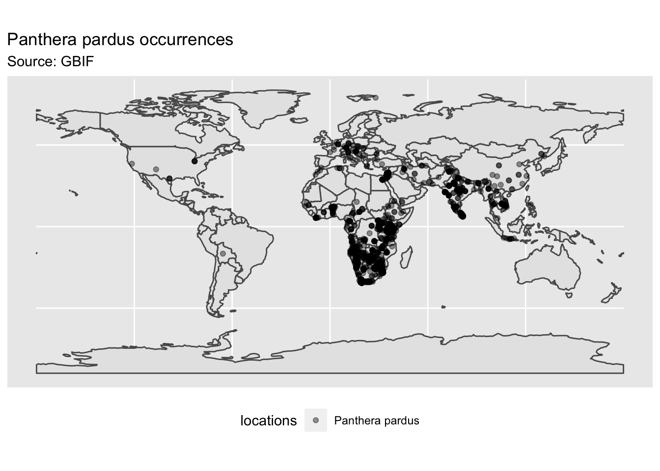
Some thoughts on the initial global map include records indicating leopards occurring in North and South America and Europe, which come as a surprise to me. These were probably occurrences in zoos or other captive facilities listed by public citizens. Thus, it is probably best to know a few things on current distribution of your focal species of interest before integrating records from public databases, such as GBIF.
However, we can create a second map that focuses on Africa and Asia continents to get a clearer look at more natural leopard occurrences. We do this by filtering the areas of interest (Africa and Asia) in our World object. We then make sure the projections for both pardus_sf_aa and africa_asia objects are the same so that we can use the st_intersection() function to clip the locations that fall outside our Africa and Asia polygon, so that points in North America, South America and Europe don’t show up on the map. The st_crs() argument is handy for extracting the CRS information from an object, and the st_transform() argument lets you change the CRS information for a given object. Changing the alpha value on the pardus_sf_aa points can show the density of locations; darker points show us that an aggregation of occurrences are mainly in southern Africa and India.
# filter world map for asia and africa continent
africa_asia <- World %>%
  filter(continent=="Africa" | continent == "Asia")
# set CRS for africa_asia the same as pardus
myCRS <- st_crs(pardus_sf)
africa_asia <- africa_asia %>%
  st_transform(myCRS)
# check CRS
st_crs(africa_asia)
## Coordinate Reference System:
##   User input: EPSG:4326
##   wkt:
## GEOGCRS["WGS 84",
##     DATUM["World Geodetic System 1984",
##         ELLIPSOID["WGS 84",6378137,298.257223563,
##             LENGTHUNIT["metre",1]]],
##     PRIMEM["Greenwich",0,
##         ANGLEUNIT["degree",0.0174532925199433]],
##     CS[ellipsoidal,2],
##         AXIS["geodetic latitude (Lat)",north,
##             ORDER[1],
##             ANGLEUNIT["degree",0.0174532925199433]],
##         AXIS["geodetic longitude (Lon)",east,
##             ORDER[2],
##             ANGLEUNIT["degree",0.0174532925199433]],
##     USAGE[
##         SCOPE["unknown"],
##         AREA["World"],
##         BBOX[-90,-180,90,180]],
##     ID["EPSG",4326]]
st_crs(pardus_sf)
## Coordinate Reference System:
##   User input: EPSG:4326
##   wkt:
## GEOGCRS["WGS 84",
##     DATUM["World Geodetic System 1984",
##         ELLIPSOID["WGS 84",6378137,298.257223563,
##             LENGTHUNIT["metre",1]]],
##     PRIMEM["Greenwich",0,
##         ANGLEUNIT["degree",0.0174532925199433]],
##     CS[ellipsoidal,2],
##         AXIS["geodetic latitude (Lat)",north,
##             ORDER[1],
##             ANGLEUNIT["degree",0.0174532925199433]],
##         AXIS["geodetic longitude (Lon)",east,
##             ORDER[2],
##             ANGLEUNIT["degree",0.0174532925199433]],
##     USAGE[
##         SCOPE["unknown"],
##         AREA["World"],
##         BBOX[-90,-180,90,180]],
##     ID["EPSG",4326]]
# now union
pardus_sf_aa <- st_intersection(pardus_sf, africa_asia)
# combine sf objects to produce ggplot map
ggplot() +
  geom_sf(data = africa_asia) +
  geom_sf(data = pardus_sf_aa, aes(color = "Panthera pardus"), alpha = 0.4) +
  labs(title = "Panthera pardus occurrences in Africa and Asia",
       subtitle = "Source: GBIF") +
  scale_color_manual(name = "locations",
                     values = "#FD7F00") +
  theme(legend.position = "bottom")
