We Out Here Tryin' to Function

I think one of the key steps in making “improvements” on your R journey is to write code that is more clear, concise and short; for me, this usually occurs when I need to create multiple plots of variables when exploring a dataset.

I find myself usually making simple bar plots using ggplot and geom_col() to count things. Instead of copying-and-pasting the same ggplot code and altering the the column names in the code like a newbie hack, I recently learned a new function that can handle the tidyverse workflow when making bar plots.

First, we’ll use the palmerpenguins package to make some bar plots (Yeah, I am fully aware that I should’ve worked with some Spotify/Apple Music Bay Area music dataset in order to make this blog post even more hyphy…). I examine the penguins dataset to see which columns are categorical/discrete and numerical/continuous:

library(tidyverse)
library(palmerpenguins)
theme_set(theme_minimal())

penguins %>% glimpse()

## Rows: 344
## Columns: 8
## $ species           <fct> Adelie, Adelie, Adelie, Adelie, Adelie, Adelie, Adel…
## $ island            <fct> Torgersen, Torgersen, Torgersen, Torgersen, Torgerse…
## $ bill_length_mm    <dbl> 39.1, 39.5, 40.3, NA, 36.7, 39.3, 38.9, 39.2, 34.1, …
## $ bill_depth_mm     <dbl> 18.7, 17.4, 18.0, NA, 19.3, 20.6, 17.8, 19.6, 18.1, …
## $ flipper_length_mm <int> 181, 186, 195, NA, 193, 190, 181, 195, 193, 190, 186…
## $ body_mass_g       <int> 3750, 3800, 3250, NA, 3450, 3650, 3625, 4675, 3475, …
## $ sex               <fct> male, female, female, NA, female, male, female, male…
## $ year              <int> 2007, 2007, 2007, 2007, 2007, 2007, 2007, 2007, 2007…

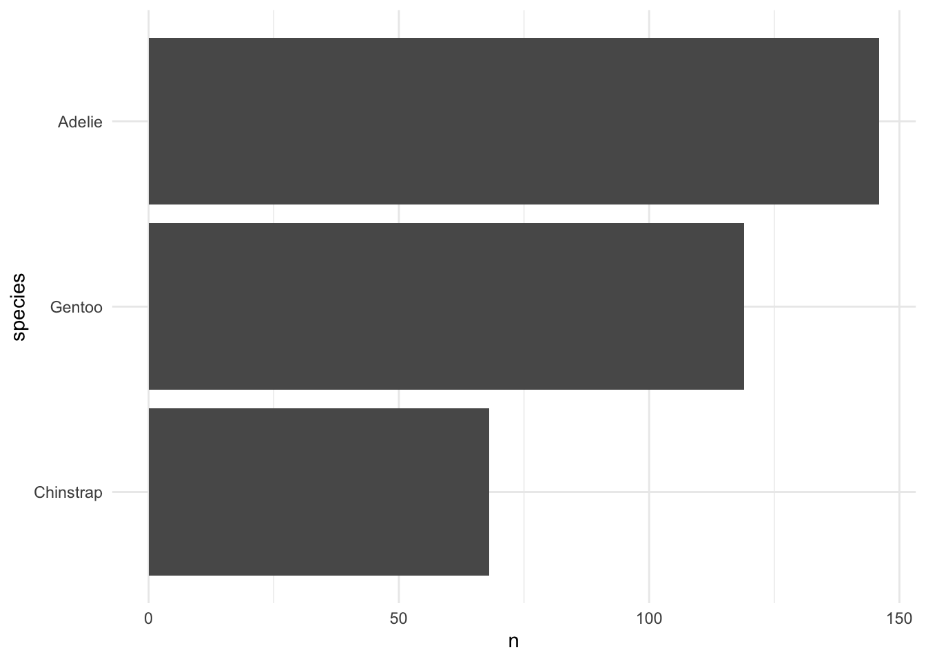
An easy first look at exploring a dataset is to simply count the number of items in a variable. I want to determine the counts across the categorical columns and make a bar plot for each. That happens to be the species, island and sex columns. Here’s the long way how to do it:

penguins %>% 
  drop_na() %>% 
  count(species, sort = TRUE) %>% 
  mutate(species = fct_reorder(species, n)) %>% 
  ggplot(aes(x = species, y = n)) + 
  geom_col() +
  coord_flip()

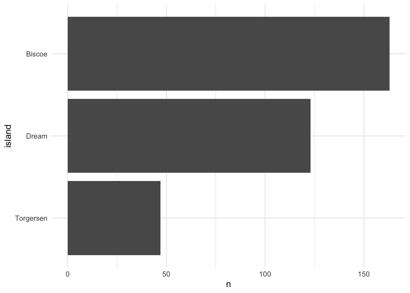
penguins %>% 
  drop_na() %>% 
  count(island, sort = TRUE) %>% 
  mutate(island = fct_reorder(island, n)) %>% 
  ggplot(aes(x = island, y = n)) + 
  geom_col() +
  coord_flip()

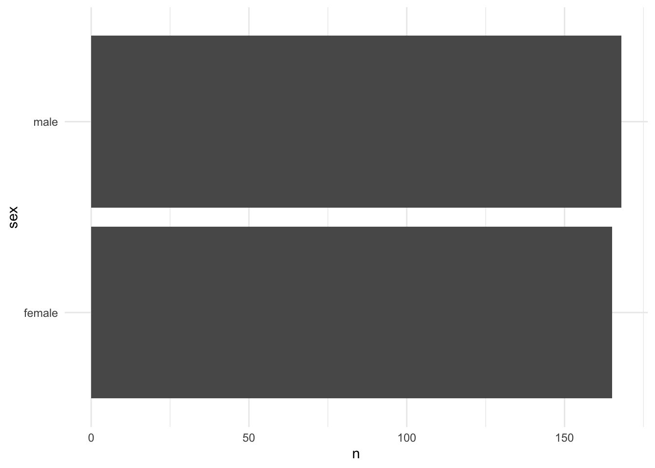
penguins %>% 
  drop_na() %>% 
  count(sex, sort = TRUE) %>% 
  mutate(sex = fct_reorder(sex, n)) %>% 
  ggplot(aes(x = sex, y = n)) + 
  geom_col() +
  coord_flip()

(There should be three plots but I’ve disabled the output for brevity’s sake). In the code demonstrated above, I realize that all I am just changing is the name of the columns (species, island, sex) to create the three different plots. The rule of thumb is to avoid duplication of code; here we can attempt to create a function to shorten the number of lines written. We can create a function (I named it geomcol_discrete) with the nifty use of double brackets {{ column }} to maintain a tidyverse work flow:

# function - discrete plots
geomcol_discrete <- function(tbl, column) {
  tbl %>% 
    drop_na() %>% 
    count({{ column }}, sort = TRUE) %>% 
    mutate({{ column }} := fct_reorder({{ column }}, n)) %>% 
    ggplot(aes(x = {{ column }}, y = n)) + 
    geom_col() +
    coord_flip()
}

# now we quickly plot
penguins %>% geomcol_discrete(species)

penguins %>% geomcol_discrete(island)

penguins %>% geomcol_discrete(sex)

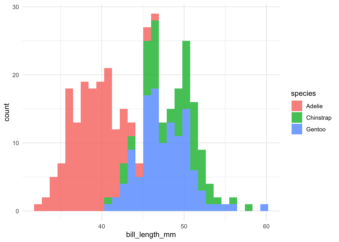
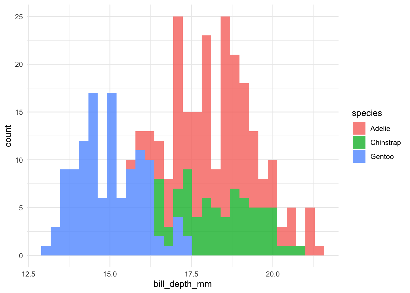
I also created a function to plot histograms for the continuous data (geomhist_continuous):

# function - continuous plots
geomhist_continuous <- function(tbl, column) {
  tbl %>% 
    drop_na() %>% 
    ggplot(aes(x = {{ column }}, fill = species)) +
    geom_histogram(alpha = 0.8)
}

# now we quickly plot
penguins %>% geomhist_continuous(bill_length_mm)

penguins %>% geomhist_continuous(bill_depth_mm)

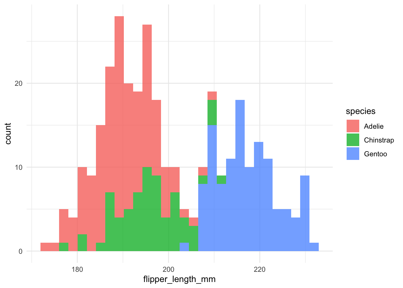
penguins %>% geomhist_continuous(flipper_length_mm)

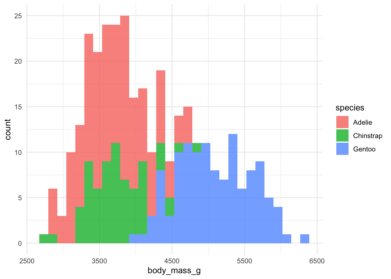
penguins %>% geomhist_continuous(body_mass_g)

The next step further would be to create a vector of column names so that I can loop the functions. Stay tuned for a future update. As the Bay Area colloquially says, “We out here tryin’ to function!”